CLIJ
GPU-accelerated image processing in ImageJ using CLIJ
Benchmarking CLIJ operations versus ImageJ/Fiji operations using JMH
In order to measure performance differences between ImageJ and CLIJ operations, we conducted benchmarking experiments. Therefore, we used the Java Microbenchmark Harness library.
Benchmarking operations
First, we set up a list of operations to benchmark in more detail. The list contains typical operations such as morphological filters, binary image operations, thresholding and projections. The operations were encapsulated in respective Benchmarking modules and put in a Java package; Each of these modules has several methods implementing different ways to call the given operation. Methods starting with ‘clij’ utilize CLIJ and the GPU. Others call ImageJ or third-party libraries to execute the operation. As executing all operations under various conditions takes a large amount of time, we executed the benchmarks on one clij operation (clij, clij_sphere or clij_box) compared to one ImageJ operation (ijrun, ijapi or vib).
All operations were benchmarked to measure the pure processing time excluding time spent for data transfer between CPU and GPU and compilation time. In order to measure pure processing times of the operations, image data transfor from/to GPU was excluded from operations benchmarking. Additionally, we measured the transfer time independently. Furthermore, Java and GPU code compilation time was excluded by ignoring the first 10 out of 20 iterations. During this so called warm-up phase, compiled code is cached and can be reused in subsequent iterations.
Compared Java code
The full list of tested operations and corresponding code is available here.
Image data
For benchmarking operations, we used images with random pixel values of pixel type 16-bit of different sizes for 2D:
- 1x1 (2B)
- 128x128 (32 kB)
- 256x256 (128 kB)
- 512x512 (512 kB)
- 600x600 (703 kB)
- 800x800 (1 MB)
- 1024x1024 (2 MB)
- 1200x1200 (3 MB)
- 1400x1400 (4 MB)
- 1600x1600 (5 MB)
- 1800x1800 (6 MB)
- 2048x2048 (8 MB)
- 3072x3072 (18 MB)
- 4096x4096 (32 MB)
and 3D:
- 1x1x1 (2B)
- 1024x1024x4 (8 MB)
- 1024x1024x8 (16 MB)
- 1024x1024x12 (24 MB)
- 1024x1024x16 (32 MB)
- 1024x1024x20 (40 MB)
- 1024x1024x24 (48 MB)
- 1024x1024x32 (64 MB)
- 1024x1024x40 (80 MB)
- 1024x1024x50 (100 MB)
- 1024x1024x64 (128 MB)
- 1024x1024x80 (160 MB)
- 1024x1024x100 (200 MB)
- 1024x1024x128 (256 MB)
For testing operations with different radii we used images with a size of
- 2048x2048 pixels (8 MB) for 2D operations and
- 1024x1024x32 voxels (64 MB) for 3D operations.
The used images are available online.
Benchmarked computing hardware
Benchmarking was executed on
- a laptop with an Intel Core i7-8650U CPU and a Intel UHD 620 GPU (“MYERS-PC-21”),
- a workstation with an Intel Xeon Silver 4110 CPU in combination with a Nvidia Quadro P6000 GPU (“MYERS-PC-22”).
Results
Transfer time
The measured median transfer times +- standard deviations show clear differences between notebook (push: 0.5 +- 0.4 GB/s, pull 0.4 +- 0.5 GB/s) and workstation (push: 1.3 +- 0.6 GB/s, pull: 1.3 +- 0.4 GB/s ) suggesting that the data transfer is faster on the workstation. The image data transfer benchmarking can be reproduced by executing the main method in this class. Then, the numbers can be retraced by executing the analyse_transfer_time.py
![]()
![]()
These plots were done with the plotCompareMachinesTransferImageSize.py script.
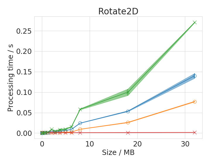
Processing time depends on image size
We chose some 2D operations to plot processing time with respect to image size in range 1B - 32 MB in detail. Benchmarking of all operations or a specific choice can be reproduced by following the instructions in the clij-benchmarking-jmh repository.
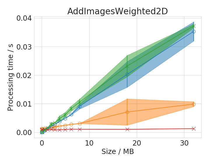
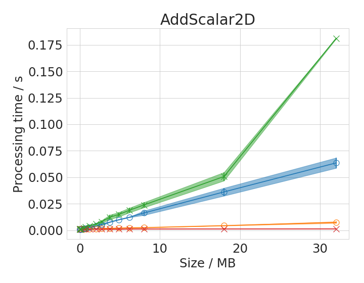
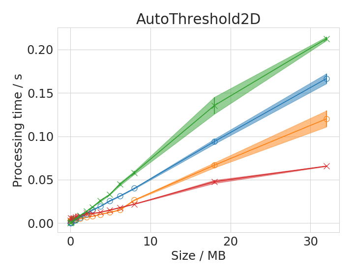
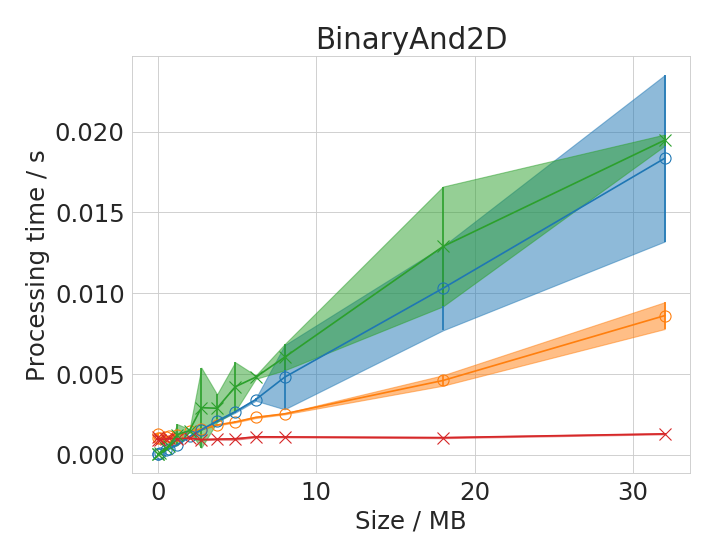
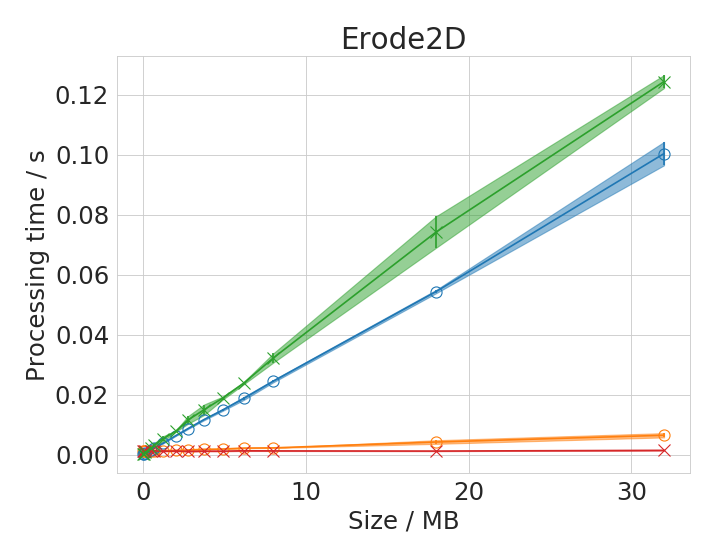
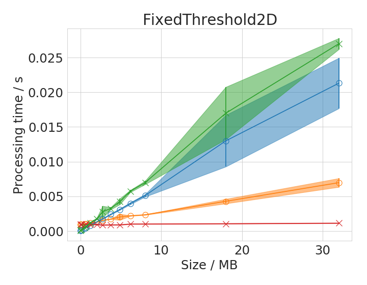
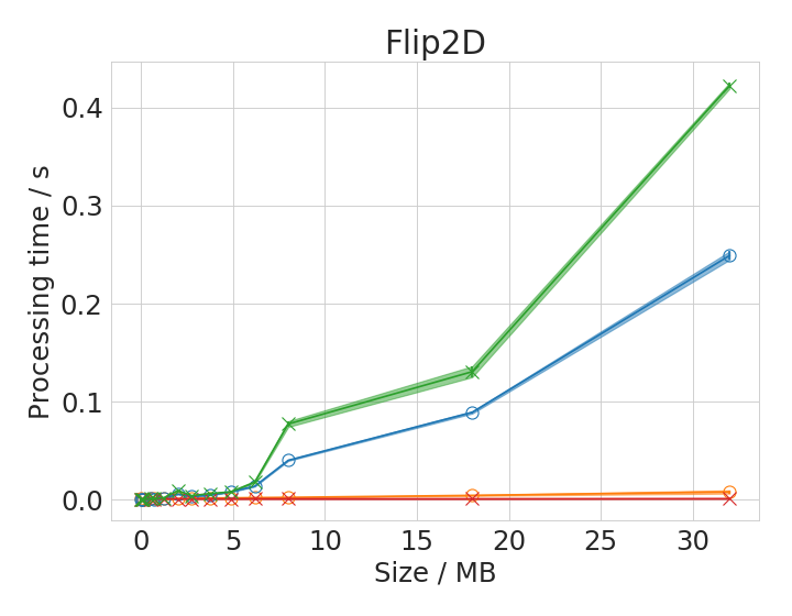
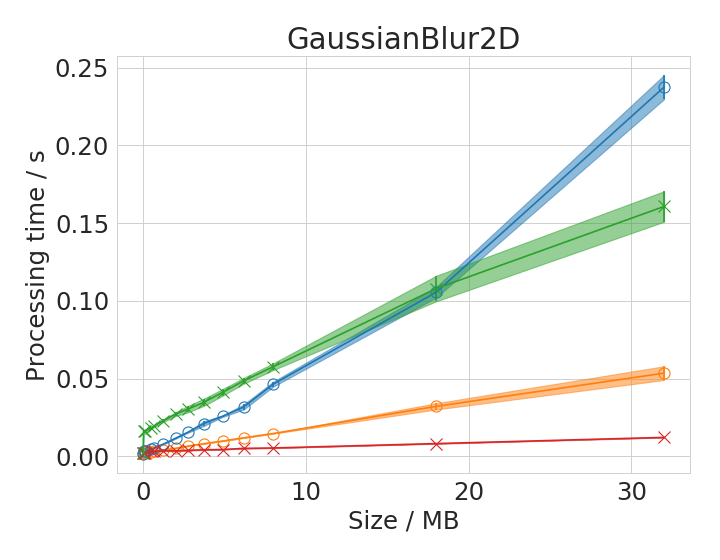
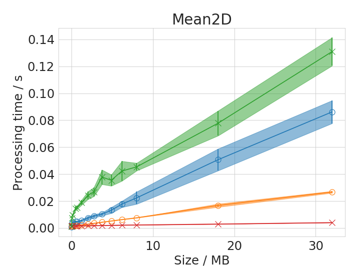
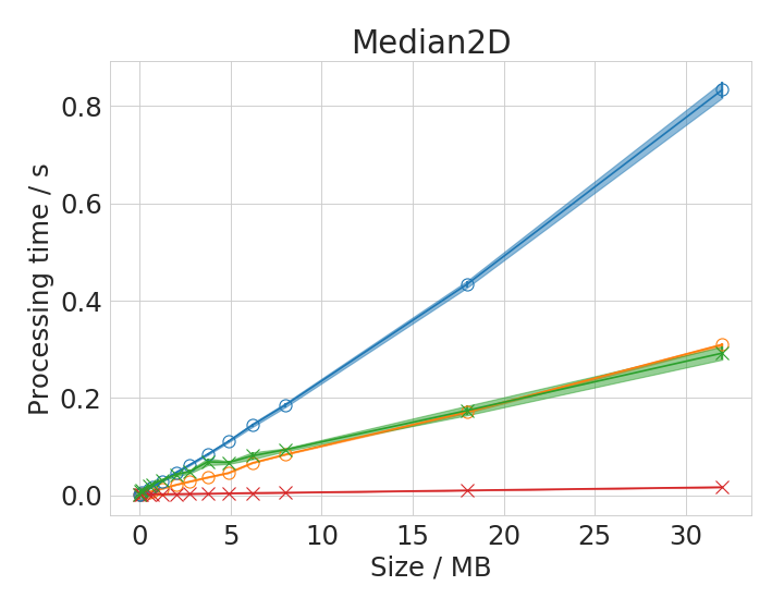
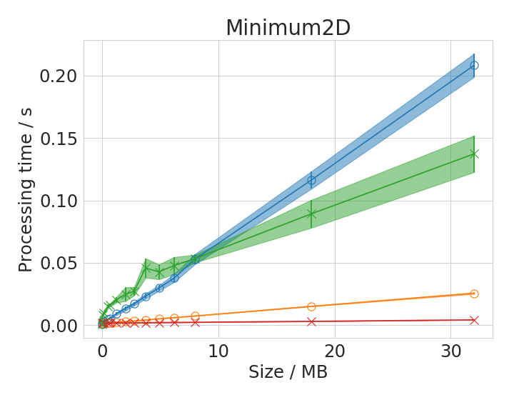
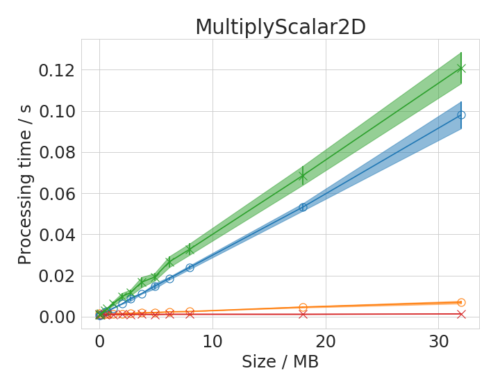

Furthermore, corresponding plots for 3D operations in image size range 1B - 128 MB:
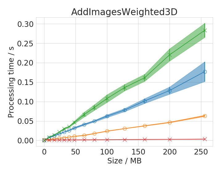
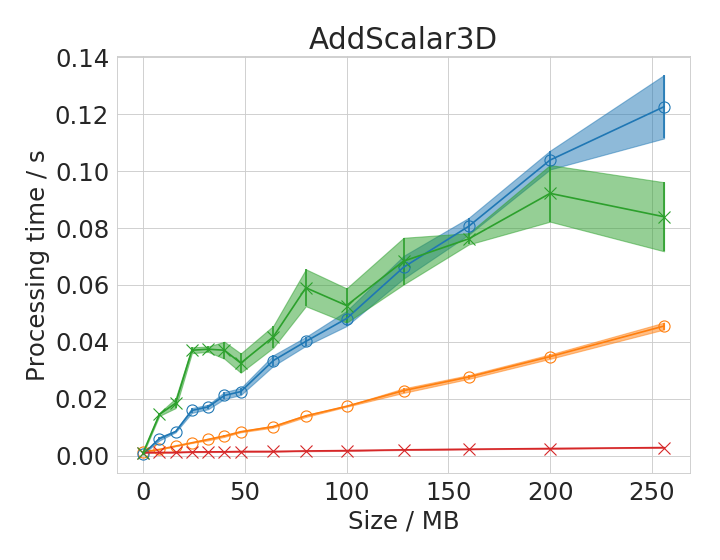
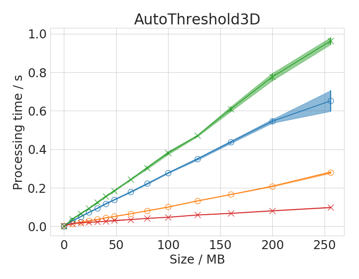
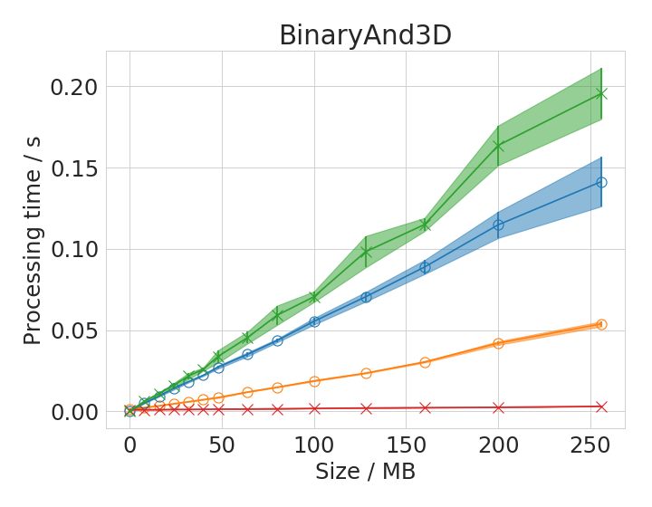
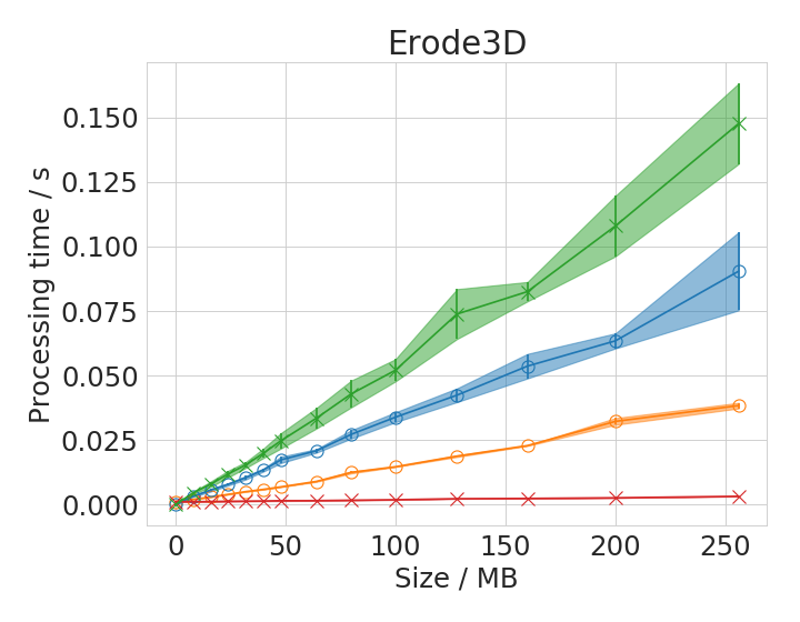
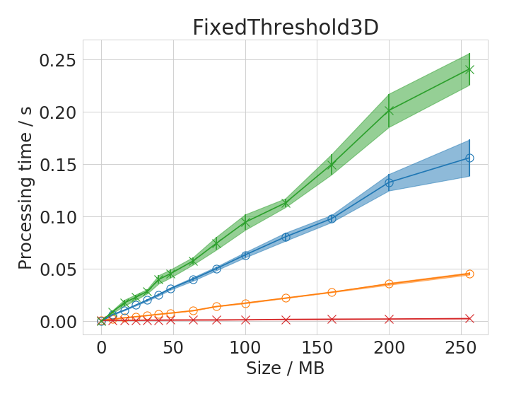
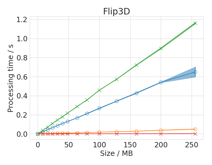
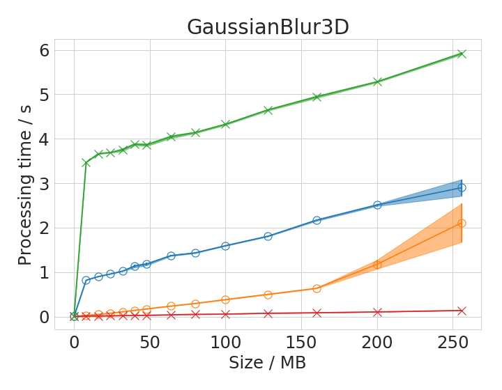
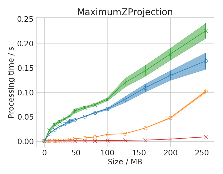
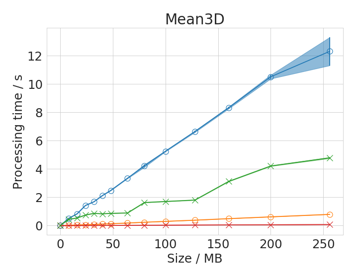
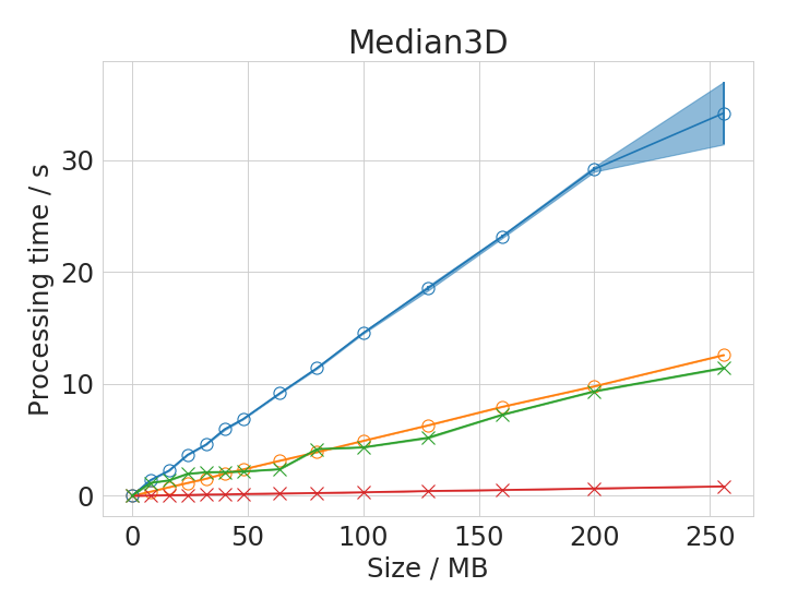
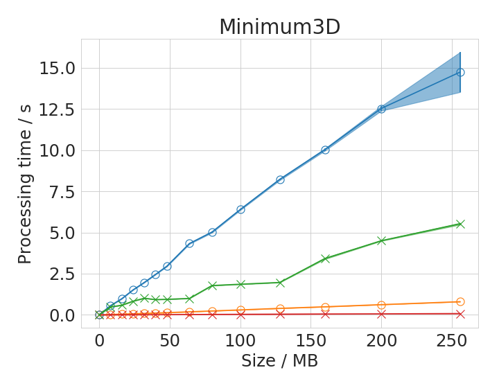
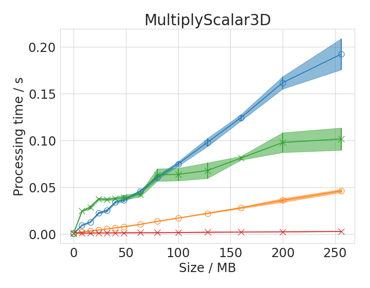
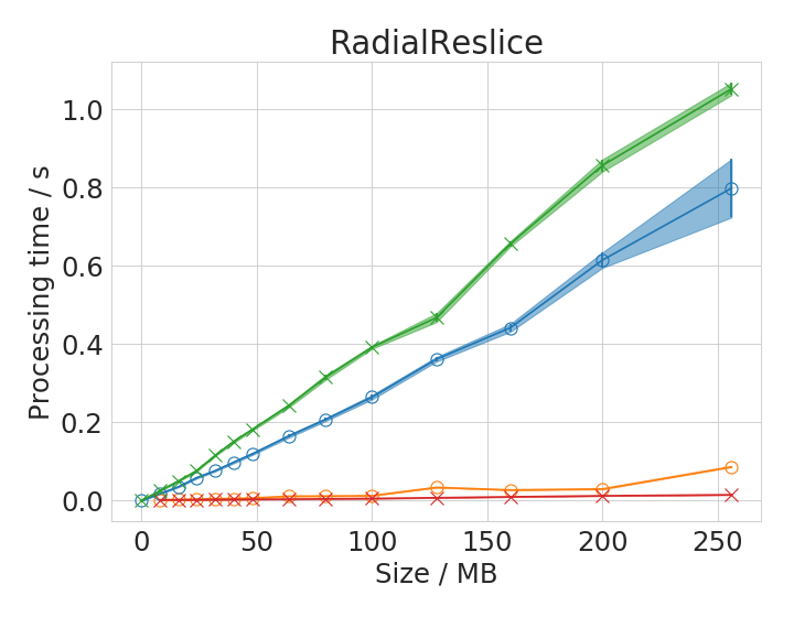
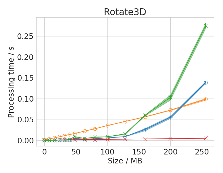
Time benchmark measurement raw data are available online; These plots were done with the plotting_ij_clij_imagesize_comparison.ipynb notebook.
Some of the operations show different behaviour with small images compared to large images. There is apparently not always a linear or polynomial relationship between image size and execution time. We assume that the cache of the CPU allows ImageJ operations running on the CPU to finish faster with small images compared to large images. This is reasonable as these caches usually hold several megabytes.
Processing time depends operation specific parameters
Some operations have parameters influencing processing time. We chose three representative examples: the Gaussian Blur filter whose processing time might depend on its sigma parameter and the Mean and the Minimum filter whose processing time might depend on the entered radius parameter.
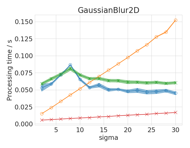
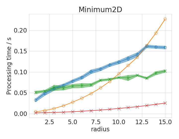
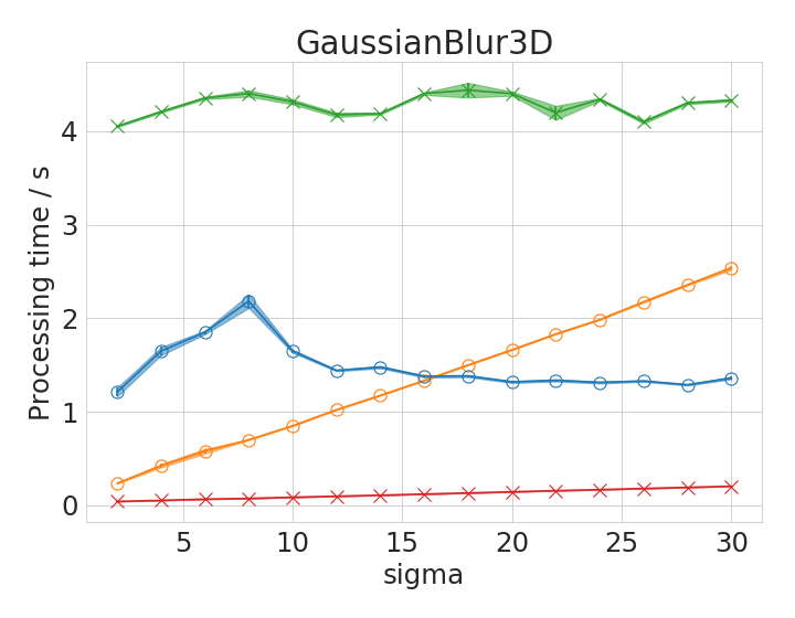
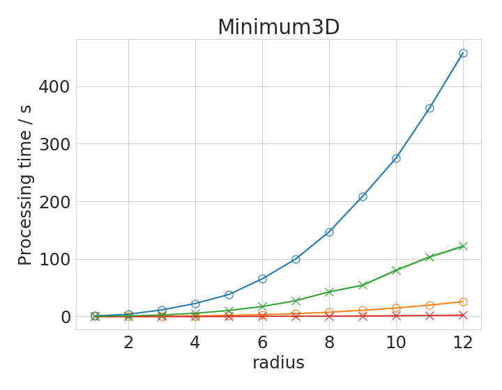
Time benchmark measurement raw data are available online: These plots were done with the plotting_ij_clij_radii_comparison.ipynb notebook.
The Gaussian Blur filter in ImageJ is optimized for speed. Apparently, it is an implementation which is independent from kernel size. Thus, with very large kernels, it can perform faster than its GPU-based counter part. The Minimum filter shows an apparently polynomial increasing time with increasing filter radius.
Speedup of operations
We also generated an overview table of speedup factors for all tested operations. The speedup was calculated relative to the ImageJ operation executed on the laptop CPU.
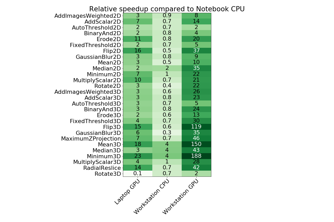
Time benchmark measurement raw data are available online. This table was generated with the speedup_table.ipynb notebook. The table shows calculated factors for image sizes of 32 MB (2D) / 64 MB (3D) and radii/sigma of 2. Speedup tables for different image sizes are available as well for 2D images and 3D images independently.
This table shows some operations to perform slower (speedup < 1) on the workstation CPU in comparison to the notebook CPU. We see the reason in the single thread performance resulting from the clock rate of the CPU. While the Intel i7-8650U is a high end mobile CPU with up to 4.2 GHz clock rate, the Intel Xeon Silver 4110 has a maximum clock rate of 3 GHz. On the other hand, there are operations shown which run faster on the workstation CPU. We assume that the algorithms implemented exploit multi-threading for higher performance yield. The workstation CPU has 8 physical cores while the laptops CPU has just 4.